polyfitter - Polynomial chain fitting and classification based on light curve morphology for binary stars
The mathematical background of polynomial chain fitting (polyfit) is published in Prša et al.,2008,ApJ,687,542. The paper that related to this code can be found Bódi&Hajdu,2021,ApJS,255,1. This code is built upon the original polyfit.
This code depends on the GNU Scientific Library (GSL) version>=2.6, which is available from here. Before installation, make sure it is properly installed, e.g. running the followings, which should return the location of the library and the installed version of GSL:
pkg-config --cflags --libs gsl && gsl-config --versionTo install the package clone this git and go the directory:
git clone https://github.com/astrobatty/polyfitter.git

cd ./polyfitter
As polyfitter is dependent on certain python package versions, the easiest way to install it is through creating a conda environment:
conda create -n polyfit python=3.7 scikit-learn=0.23.2 cython=0.29.20

conda activate polyfit

python setup.py install
If the code is not used, the environment can be deactivated:
conda deactivateIf you want to access this environment from jupyter you can do the followings:
conda install -c anaconda ipykernel

python -m ipykernel install --user --name=polyfit
Then after restarting your jupyter you'll be able to select this kernel.
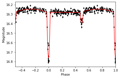
To fit a polynomial chain to the light curve of OGLE-BLG-ECL-040474:
from polyfitter import Polyfitter

import numpy as np

# Parameters from OGLE database
ID = 'OGLE-BLG-ECL-040474'
P  = 1.8995918
t0 = 7000.90650

# Load light curve from OGLE database
# This is in magnitude scale
path_to_ogle = 'http://ogledb.astrouw.edu.pl/~ogle/OCVS/data/I/'+ID[-2:]+'/'+ID+'.dat'
lc = np.loadtxt(path_to_ogle).T

# For clarity
time = lc[0]
mag  = lc[1]
err  = lc[2]

# Create Polyfitter instance by setting the brightness scale of your data
# Set scale to "mag" or "flux"
pf = Polyfitter(scale='mag')

# Run polynomial chain fitting
t0new, phase, polyfit, messages = pf.get_polyfit(time,mag,err,P,t0)
Plotting our results gives:
import matplotlib.pyplot as plt

plt.errorbar((time-t0new)/P%1,mag,err,fmt='k.')
plt.errorbar((time-t0new)/P%1-1,mag,err,fmt='k.')
plt.plot(phase,polyfit,c='r',zorder=10)
plt.plot(phase+1,polyfit,c='r',zorder=10)
plt.xlabel('Phase')
plt.ylabel('Magnitude')
plt.xlim(-0.5,1)
plt.gca().invert_yaxis()
plt.show()
And the morphology classification:
morp_array = pf.c
print('Morphology type =' , morp_array[0] )
You can find a Google Colab friendly tutorial in the examples.
The difference from using the code interactively is that you have to put your code under a main function. See here how to do it.
-
Polyfitter class instance:
scaleThe scale of the input data that will be used with this instance. Must be "mag" or "flux".debugIfTrueeach fit will be displayed with auxiliary messages.
-
Getting polyfit:
verboseIf0the fits will be done silently. Default is1.verticesNumber of equidistant vertices in the computed fit. Default is1000, which is mandatory to run the classification afterwards.maxitersMaximum number of iterations. Default is4000.timeoutThe time in seconds after a fit will be terminated. Default is100.
Feel free to open PR / Issue.
If you find this code useful, please cite Bódi&Hajdu,2021,ApJS,255,1, and Prša et al.,2008,ApJ,687,542. Here are the BibTeX sources:
@ARTICLE{2021ApJS..255....1B,
       author = {{B{\'o}di}, A. and {Hajdu}, T.},
        title = "{Classification of OGLE Eclipsing Binary Stars Based on Their Morphology Type with Locally Linear Embedding}",
      journal = {\apjs},
     keywords = {Eclipsing binary stars, Astronomy data analysis, Astronomy databases, 444, 1858, 83, Astrophysics - Solar and Stellar Astrophysics, Astrophysics - Instrumentation and Methods for Astrophysics},
         year = 2021,
        month = jul,
       volume = {255},
       number = {1},
          eid = {1},
        pages = {1},
          doi = {10.3847/1538-4365/ac082c},
archivePrefix = {arXiv},
       eprint = {2106.01039},
 primaryClass = {astro-ph.SR},
       adsurl = {https://ui.adsabs.harvard.edu/abs/2021ApJS..255....1B},
      adsnote = {Provided by the SAO/NASA Astrophysics Data System}
}

@ARTICLE{2008ApJ...687..542P,
       author = {{Pr{\v{s}}a}, A. and {Guinan}, E.~F. and {Devinney}, E.~J. and {DeGeorge}, M. and {Bradstreet}, D.~H. and {Giammarco}, J.~M. and {Alcock}, C.~R. and {Engle}, S.~G.},
        title = "{Artificial Intelligence Approach to the Determination of Physical Properties of Eclipsing Binaries. I. The EBAI Project}",
      journal = {\apj},
     keywords = {methods: data analysis, methods: numerical, binaries: eclipsing, stars: fundamental parameters, Astrophysics},
         year = 2008,
        month = nov,
       volume = {687},
       number = {1},
        pages = {542-565},
          doi = {10.1086/591783},
archivePrefix = {arXiv},
       eprint = {0807.1724},
 primaryClass = {astro-ph},
       adsurl = {https://ui.adsabs.harvard.edu/abs/2008ApJ...687..542P},
      adsnote = {Provided by the SAO/NASA Astrophysics Data System}
}
This project was made possible by the funding provided by the Lendület Program of the Hungarian Academy of Sciences, project No. LP2018-7.


