Monte Carlo Simulation for Radiation View Factors of Two Geometries

Between two objects, the proportion of the radiation that leaves one object and hits the other object, is called the Radiation View Factor. There are a variety of techniques to calculate the view factor of an object with respect to another. Some references contain analytic methods for certain geometries, while others investigate the use of numerical methods for more complex geometries. In this code, the Monte Carlo Method is used to simulate emissions, and to compute the view factors. More specifically, this code runs a Monte Carlo simulation for a 3D geometry of two co-axial parallel disks, then plots the results and compares them with the actual (analytic) values presented in references, and observes the relationship of errors and radii of each disk.

Running the tests

MATLAB is required in order to run the scripts, works with all versions of MATLAB.

2D Geometry: Equilateral Triangle

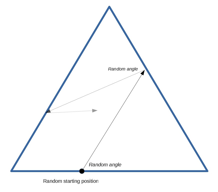
This is the simplest geometry to run Monte Carlo Simulation on. It does not have the complications of 3D geometries and therefore it's suitable for learning the basics of Monte Carlo in heat transfer. Run the script on the main directory to do this:

Triangle_MonteCarlo

How it works

As can be seen in the above figure, continuous radiations are emitted from surface 1 and hit the two other surfaces. The position and angle at which the radiation is emitted is determined by a random number. Then, the radiation hits another surface. With a probability of absoption of 1/2, the radiation is either absorbed or reflected from the surface. If the radiation is absorbed, the result is saved and simulation restarts with another random radiation from surface 1. If not, the radiation continues to bounce between walls of the triangle until it is absorbed eventually.

Results

According to the references, surface 1 (from which continuous radiation is emitted) should have a view factor of 0.2, this leaves the other two surfaces with equal shares of 0.4 each. After you run the code, the results should look be reported like below:

Starting Simulation...
Simulation Done. Total number of simulations: 10000
2074 radiations hit surface 1, Radiation View Factor = 0.21, error: 0.74%
4005 radiations hit surface 2, Radiation View Factor = 0.40, error: 0.05%
3921 radiations hit surface 3, Radiation View Factor = 0.39, error: -0.79%

So the overall error of the Monte Carlo method with 10,000 simulations is less than 1%.

3D Geometry: Two Coaxial Parallel Disks

Two Coaxial Parallel Disks with different diameters that are in distance L from each other. The simulation is done as explained above but this time with more random variables. Therefore, the simulation needs to be run more times in order for the results to converge. You may choose to run the Monte Carlo simulation in Cylindrical_MonteCarlo which will take some time, or simply see the detailed results by executing the script below:

Cylindrical_Results_Detailed

Results and Analysis

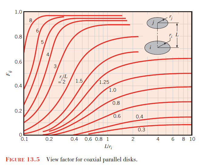
Below is a figure from the book "Introduction to Heat Transfer" by Bergman:

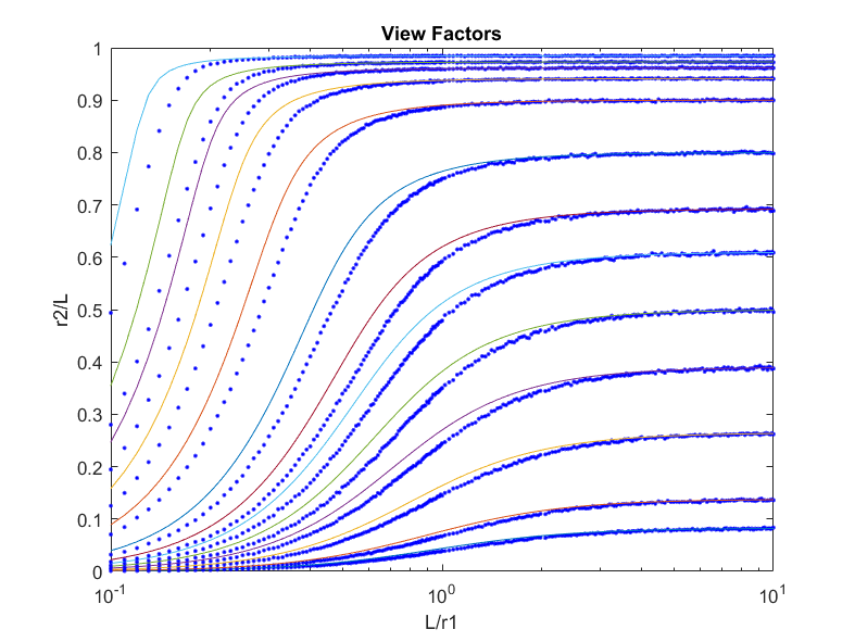
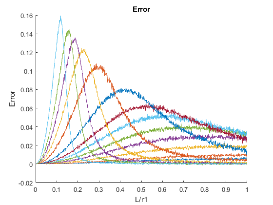
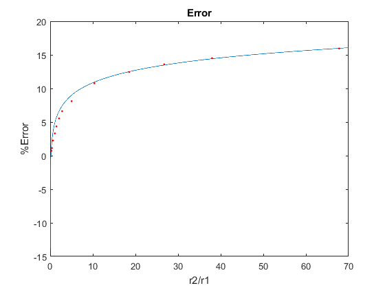
Which shows the analytic results with respect to the values r1, r2 and L. We'll reproduce the same figure in MATLAB and compare the analytic results with the results obtained by the Monte Carlo method, which should look like this:

Where colored lines are for different r2/L values just like the previous figure, and blue dots show the corresponding results from the Monte Carlo method. There seems to be a difference in error over time between the lines. In other words, the Monte Carlo dots start off close to the real values, deviate from the lines, and eventually converge to the analytic values. We can investigate this phenomenon by plotting the error between the analytic and Monte Carlo methods for each line:

In this plot we can see the distribution of error for each of the lines over time, which show just what we expected. Moreover, we can see that the peak of these lines (where maximum error happens) have a relationship to the ratio of the diameters of two disks. The next figure illustrates this by fitting an exponential function to the *"max error"* plot:

Notes

In the code, the default ranges of values for diameters of disks (r1 & r2) are considered according to the reference. If a different precision is needed in plots, you may manually change the range of r1 and r2 values.

License

This project is licensed under the MIT License - Author: Abdolreza Taheri

Contribute

Any contribution in further reducing the error of the monte carlo simulation is appreciated (see the error plot), please don't hesitate to contribute or make suggestions.