statisticalmodels_20191202_166_hwa.rmd

---
title: "16.4 Bayesian statistics"
output: html_notebook
---

What does it mean when an election forecaster tells us that a given candidate has a 90% chance of winning? In the context of the urn model, this would be equivalent to stating that the probability $p>0.5$ is 90%. However, as we discussed earlier, in the urn model $p$ is a fixed parameter and it does not make sense to talk about probability. With Bayesian statistics, we model $p$ as random variable and thus a statement such as "90% chance of winning" is consistent with the approach.

Forecasters also use models to describe variability at different levels. For example, sampling variability, pollster to pollster variability, day to day variability, and election to election variability. One of the most successful approaches used for this are hierarchical models, which can be explained in the context of Bayesian statistics.

In this chapter we briefly describe Bayesian statistics. For an in-depth treatment of this topic we recommend one of the following textbooks:

* Berger JO (1985). Statistical Decision Theory and Bayesian Analysis, 2nd edition. Springer-Verlag. 

* Lee PM (1989). Bayesian Statistics: An Introduction. Oxford. 

### 16.4.1 Bayes theorem

We start by describing Bayes theorem. We do this using a hypothetical cystic fibrosis test as an example. 
Suppose a test for cystic fibrosis has an accuracy of 99%. We will use the following notation:

$$
\mbox{Prob}(+ \mid D=1)=0.99, \mbox{Prob}(- \mid D=0)=0.99 
$$

with $+$ meaning a positive test and $D$ representing if you actually have the disease (1) or not (0).

Suppose we select a random person and they test positive. What is the probability that they have the disease?  We write this as $\mbox{Prob}(D=1 \mid +)?$ The cystic fibrosis rate is 1 in 3,900 which implies that  $\mbox{Prob}(D=1)=0.00025$. To answer this question, we will use Bayes theorem, which in general tells us that:

$$
\mbox{Pr}(A \mid B)  =  \frac{\mbox{Pr}(B \mid A)\mbox{Pr}(A)}{\mbox{Pr}(B)} 
$$

This equation applied to our problem becomes:

$$
\begin{aligned}
\mbox{Pr}(D=1 \mid +) & =  \frac{ P(+ \mid D=1) \cdot P(D=1)} {\mbox{Pr}(+)} \\
& =  \frac{\mbox{Pr}(+ \mid D=1)\cdot P(D=1)} {\mbox{Pr}(+ \mid D=1) \cdot P(D=1) + \mbox{Pr}(+ \mid D=0) \mbox{Pr}( D=0)} 
\end{aligned}
$$

Plugging in the numbers we get:

$$
\frac{0.99 \cdot 0.00025}{0.99 \cdot 0.00025 + 0.01 \cdot (.99975)}  =  0.02 
$$

This says that despite the test having 0.99 accuracy, the probability of having the disease given a positive test is only 0.02. This may appear counter-intuitive to some, but the reason this is the case is because we have to factor in the very rare probability that a person, chosen at random, has the disease. To illustrate this, we run a Monte Carlo simulation.

# 16.5 Bayes theorem simulation

The following simulation is meant to help you visualize Bayes theorem. We start by randomly selecting 100,000 people from a population in which the disease in question has a 1 in 4,000 prevalence.

```{r}
prev <- 0.00025
N <- 100000
outcome <- sample(c("Disease","Healthy"), N, replace = TRUE, 
                  prob = c(prev, 1 - prev))
```

Note that there are very few people with the disease:

```{r}
N_D <- sum(outcome == "Disease")
N_D
N_H <- sum(outcome == "Healthy")
N_H
```

Also, there are many without the disease, which makes it more probable that we will see some false positives given that the test is not perfect. Now each person gets the test, which is correct 99% of the time:

```{r}
accuracy <- 0.99
test <- vector("character", N)
test[outcome == "Disease"]  <- sample(c("+", "-"), N_D, replace = TRUE, 
                                    prob = c(accuracy, 1 - accuracy))
test[outcome == "Healthy"]  <- sample(c("-", "+"), N_H, replace = TRUE, 
                                    prob = c(accuracy, 1 - accuracy))
```

Because there are so many more controls than cases, even with a low false positive rate we get more controls than cases in the group that tested positive:


```{r}
table(outcome, test)
```

From this table, we see that the proportion of positive tests that have the disease is 22 out of 968. We can run this over and over again to see that, in fact, the probability converges to about 0.022.


### 16.5.1 Bayes in practice


José Iglesias is a professional baseball player. In April 2013, when he was starting his career, he was performing rather well:

| Month | At Bats | H | AVG |
|-------|---------|---|-----|
| April | 20      | 9 | .450|

The batting average (`AVG`) statistic is one way of measuring success. Roughly speaking, it tells us the success rate when batting. An `AVG` of .450 means José has been successful 45% of the times he has batted (`At Bats`) which is rather high, historically speaking. Keep in mind that no one has finished a season with an `AVG` of .400 or more since Ted Williams did it in 1941! To illustrate the way hierarchical models are powerful, we will try to predict José's batting average at the end of the season. Note that in a typical season, players have about 500 at bats.

With the techniques we have learned up to now, referred to as _frequentist techniques_, the best we can do is provide a confidence interval. We can think of outcomes from hitting as a binomial with a success rate of $p$. So if the success rate is indeed .450, the standard error of just 20 at bats is:

$$
\sqrt{\frac{.450 (1-.450)}{20}}=.111
$$

This means that our confidence interval is $.450 - .222$ to $.450 + .222$ or $.228$ to $.672$.

This prediction has two problems. First, it is very large, so not very useful. Second, it is centered at .450, which implies that our best guess is that this new player will break Ted Williams' record. 

If you follow baseball, this last statement will seem wrong and this is because you are implicitly using a hierarchical model that factors in information from years of following baseball. Here we show how we can quantify this intuition.

First, let's explore the distribution of batting averages for all players with more than 500 at bats during the previous three seasons:
![batavgthreeseasons](https://rafalab.github.io/dsbook/book_files/figure-html/batting-averages-histogram-1.png)


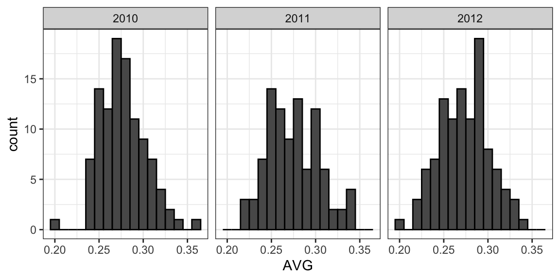
The average player had an `AVG` of .275 and the standard deviation of the population of players was 0.027. So we can see already that .450 would be quite an anomaly since it is over six standard deviations away from the mean. 

So is José lucky or is he the best batter seen in the last 50 years? Perhaps it's a combination of both luck and talent. But how much of each? If we become convinced that he is lucky, we should trade him to a team that trusts the .450 observation and is maybe overestimating his potential.

# 16.6 Hierarchial models

The hierarchical model provides a mathematical description of how we came to see the observation of .450. First, we pick a player at random with an intrinsic ability summarized by, for example, $p$. Then we see 20 random outcomes with success probability $p$.

We use a model to represent two levels of variability in our data. First, each player is assigned a natural ability to hit. We will use the symbol $p$ to represent this ability. You can think of $p$ as the batting average you would converge to if this particular player batted over and over again. 

Based on the plots we showed earlier, we assume that $p$ has a normal distribution. With expected value .270 and standard error 0.027. 

Now the second level of variability has to do with luck when batting. Regardless of how good the player is, sometimes you have bad luck and sometimes you have good luck. At each at bat, this player has a probability of success $p$. If we add up these successes and failures, then the CLT tells us that the observed average, call it $Y$, has a normal distribution with expected value $p$ and standard error $\sqrt{p(1-p)/N}$ with $N$ the number of at bats.

Statistical textbooks will write the model like this:
$$
\begin{aligned}
p &\sim N(\mu, \tau^2) \\
Y \mid p &\sim N(p, \sigma^2) 
\end{aligned}
$$
Here the $\sim$ symbol tells us the random variable on the left of the symbol follows the distribution on the right and $N(a,b^2)$ represents the normal distribution with mean $a$ and standard deviation $b$. The $\mid$ is read as _conditioned on_, and it means that we are treating the random variable to the right of the symbol as known. We refer to the model as hierarchical because we need to know $p$, the first level, in order to model $Y$, the second level. In our example the first level describes randomness in assigning talent to a player and the second describes randomness in this particular player's performance once we have fixed the talent parameter. In a Bayesian framework, the first level is called a _prior distribution_ and the second the _sampling distribution_. The data analysis we have conducted here suggests that we set $\mu = .270$, $\tau = 0.027$, and $\sigma^2 = p(1-p)/N$.

Now, let's use this model for José's data. Suppose we want to predict his innate ability in the form of his _true_ batting average $p$. This would be the hierarchical model for our data:

$$
\begin{aligned}
p &\sim N(.275, .027^2) \\
Y \mid p &\sim N(p, .111^2) 
\end{aligned}
$$

We now are ready to compute a posterior distribution to summarize our prediction of $p$. The continuous version of Bayes' rule can be used here to derive the _posterior probability function_, which is the distribution of $p$ assuming we observe $Y=y$. In our case, we can show that when we fix $Y=y$, $p$ follows a normal distribution with expected value:

$$
\begin{aligned}
\mbox{E}(p \mid Y=y) &= B \mu + (1-B) y\\
&= \mu + (1-B)(y-\mu)\\
\mbox{with } B &= \frac{\sigma^2}{\sigma^2+\tau^2}
\end{aligned}
$$

This is a weighted average of the population average $\mu$ and the observed data $y$. The weight depends on the SD of the population $\tau$ and the SD of our observed data $\sigma$. This weighted average is sometimes referred to as _shrinking_ because it _shrinks_ estimates towards a prior mean. In the case of José Iglesias, we have:

$$
\begin{aligned}
\mbox{E}(p \mid Y=.450) &= B \times .275 + (1 - B) \times .450 \\
&= .275 + (1 - B)(.450 - .275) \\
B &=\frac{.111^2}{.111^2 + .027^2} = 0.944\\
\mbox{E}(p \mid Y=450) &\approx .285
\end{aligned}
$$

We do not show the derivation here, but the standard error can be shown to be:

$$
\mbox{SE}(p\mid y)^2 = \frac{1}{1/\sigma^2+1/\tau^2}
= \frac{1}{1/.111^2 + 1/.027^2} = 0.00069
$$
and the standard deviation is therefore $0.026$. So we started with a frequentist 95% confidence interval that ignored data from other players and summarized just José's data: .450 $\pm$ 0.220. Then we used a Bayesian approach that incorporated data from other players and other years to obtain a posterior probability. This is actually referred to as an empirical Bayes approach because we used data to construct the prior. From the posterior, we can report what is called a 95% _credible interval_ by reporting a region, centered at the mean, with a 95% chance of occurring. In our case, this turns out to be: .285 $\pm$ 0.052.

The Bayesian credible interval suggests that if another team is impressed by the .450 observation, we should consider trading José as we are predicting he will be just slightly above average. Interestingly, the Red Sox traded José to the Detroit Tigers in July. Here are the José Iglesias batting averages for the next five months: 

|Month|At Bat| Hits| AVG |
|-----|------|-----|-----|
|April|20|9|.450|
|May|26|11|.423|
|June|86|34|.395|
|July|83|17|.205|
|August|85|25|.294|
|September|50|10|.200|
|Total w/o April|330|97|.293|

Although both intervals included the final batting average, the Bayesian credible interval provided a much more precise prediction. In particular, it predicted that he would not be as good during the remainder of the season.

# 16.7 Exercises

1\. In 1999, in England, Sally Clark was found guilty of the murder of two of her sons. Both infants were found dead in the morning, one in 1996 and another in 1998. In both cases, she claimed the cause of death was sudden infant death syndrome (SIDS). No evidence of physical harm was found on the two infants so the main piece of evidence against her was the testimony of Professor Sir Roy Meadow, who testified that the chances of two infants dying of SIDS was 1 in 73 million. He arrived at this figure by finding that the rate of SIDS was 1 in 8,500 and then calculating that the chance of two SIDS cases was 8,500 $\times$ 8,500 $\approx$ 73 million. Which of the following do you agree with?
    
a. Sir Meadow assumed that the probability of the second son being affected by SIDS was independent of the first son being affected, thereby ignoring possible genetic causes. If genetics plays a role then: $\mbox{Pr}(\mbox{second case of SIDS} \mid \mbox{first case of SIDS}) < \mbox{P}r(\mbox{first case of SIDS})$.
b. Nothing. The multiplication rule always applies in this way: $\mbox{Pr}(A \mbox{ and } B) =\mbox{Pr}(A)\mbox{Pr}(B)$
c. Sir Meadow is an expert and we should trust his calculations.
d. Numbers don't lie.

Answer: **A**    
    
    
2\. Let's assume that there is in fact a genetic component to SIDS and the probability of $\mbox{Pr}(\mbox{second case of SIDS} \mid \mbox{first case of SIDS}) = 1/100$, is much higher than 1 in 8,500. What is the probability of both of her sons dying of SIDS?

```{r}
Prob_1 <- 1/8500
Prob_2 <- 1/100
Prob_1 * Prob_2
```


3\. Many press reports stated that the expert claimed the probability of Sally Clark being innocent as 1 in 73 million. Perhaps the jury and judge also interpreted the testimony this way. This probability can be written as the probability of _a mother is a son-murdering psychopath_ given that 
_two of her children are found dead with no evidence of physical harm_. 
According to Bayes' rule, what is this?

Answer: $$\ \frac{\mbox{Pr}(\mbox{two children found dead with no evidence of harm} \mid \mbox{mother is a murderer} ) \mbox{Pr}(\mbox{mother is a murderer})}{\mbox{Pr}(\mbox{two children found dead with no evidence of harm})}$$

4\. Assume that the chance of a son-murdering psychopath finding a way to kill her children, without leaving evidence of physical harm, is:

$$
\mbox{Pr}(A \mid B) = 0.50
$$ 

with A = two of her children are found dead with no evidence of physical harm and B = a mother is a son-murdering psychopath = 0.50. Assume that the rate of son-murdering psychopaths mothers is 1 in 1,000,000.  According to Bayes' theorem, what is the probability of $\mbox{Pr}(B \mid A)$ ?

```{r}
Prob_B <- Prob_1 * Prob_2
Prob_A <- 1/1000000
Prob_BA <- 0.50
Prob_AB <- Prob_BA*Prob_A/Prob_B
Prob_AB
```


5/. After Sally Clark was found guilty, the Royal Statistical Society issued a statement saying that there was "no statistical basis" for the expert's claim. They expressed concern at the "misuse of statistics in the courts". Eventually, Sally Clark was acquitted in June 2003. What did the expert miss?
    
a. He made an arithmetic error.
b. He made two mistakes. First, he misused the multiplication rule and did not take into account how rare it is for a mother to murder her children. After using Bayes' rule, we found a probability closer to 0.5 than 1 in 73 million.
c. He mixed up the numerator and denominator of Bayes' rule.
d. He did not use R.

Answer: **B**
    
6\. Florida is one of the most closely watched states in the U.S. election because it has many electoral votes, and the election is generally close, and Florida tends to be a swing state that can vote either way. Create the following table with the polls taken during the last two weeks:

```{r}
library(tidyverse)
library(dslabs)
data(polls_us_election_2016)
polls <- polls_us_election_2016 %>% 
  filter(state == "Florida" & enddate >= "2016-11-04" ) %>% 
  mutate(spread = rawpoll_clinton/100 - rawpoll_trump/100)
```

Take the average spread of these polls. The CLT tells us this average is approximately normal. Calculate an average and provide an estimate of the standard error. Save your results in an object called `results`.

```{r}
results <- polls %>% summarize(avg = mean(spread),  se = sd(spread)/sqrt(n()))
results
```


7\. Now assume a Bayesian model that sets the prior distribution for Florida's election night spread $d$ to be Normal with expected value $\mu$ and standard deviation $\tau$. What are the interpretations of $\mu$ and $\tau$?
    
a. $\mu$ and $\tau$ are arbitrary numbers that let us make probability statements about $d$.
b. $\mu$ and $\tau$ summarize what we would predict for Florida before seeing any polls. Based on past elections, we would set $\mu$ close to 0 because both Republicans and Democrats have won, and $\tau$ at about $0.02$, because these elections tend to be close.
c. $\mu$ and $\tau$ summarize what we want to be true. We therefore set $\mu$ at $0.10$ and $\tau$ at $0.01$. 
d. The choice of prior has no effect on Bayesian analysis.
    
Answer: **B**
    
8\. The CLT tells us that our estimate of the spread $\hat{d}$ has normal distribution with expected value $d$ and standard deviation $\sigma$ calculated in problem 6. Use the formulas we showed for the posterior distribution to calculate the expected value of the posterior distribution if we set $\mu = 0$ and $\tau = 0.01$.

```{r}
mu <- 0
tau <- 0.01
sigma <- results$se
Y <- results$avg
B <- sigma^2 / (sigma^2 + tau^2)
B
mu + (1 - B) * (Y - mu)
```


9\. Now compute the standard deviation of the posterior distribution.
```{r}
sqrt(1 / (1 / sigma ^2 + 1 / tau ^2))
```


10\. Using the fact that the posterior distribution is normal, create an interval that has a 95% probability of occurring centered at the posterior expected value. Note that we call these credible intervals.
```{r}
x <- B * mu + (1 - B) * Y
sd <- sqrt(1 / (1 / sigma ^2 + 1 / tau ^2))
ci <- c(x - qnorm(0.975) * sd, x + qnorm(0.975) * sd)
ci
```


11\. According to this analysis, what was the probability that Trump wins Florida?
```{r}
pnorm(0, x, sd)
```

12\. Now use `sapply` function to change the prior variance from `seq(0.05, 0.05, len = 100)` and observe how the probability changes by making a plot.
```{r}
tau_var <- seq(0.005, 0.05, len = 100)
calc <- function(tau){
  B <- sigma ^ 2 / (sigma^2 + tau^2)
  sd <- sqrt(1 / (1/sigma^2 + 1/tau^2))
  x <- B * mu + (1 - B) * Y
  pnorm(0, x, sd)
}
p <- sapply(tau_var, calc)
plot(tau_var, p)
```

# 16.8 Case study: election forecasting

In a previous section, we generated these data tables:
```{r}
library(tidyverse)
library(dslabs)
polls <- polls_us_election_2016 %>% 
  filter(state == "U.S." & enddate >= "2016-10-31" &
           (grade %in% c("A+","A","A-","B+") | is.na(grade))) %>% 
  mutate(spread = rawpoll_clinton/100 - rawpoll_trump/100)
one_poll_per_pollster <- polls %>% group_by(pollster) %>% 
  filter(enddate == max(enddate)) %>%
  ungroup()
results <- one_poll_per_pollster %>% 
  summarize(avg = mean(spread), se = sd(spread)/sqrt(length(spread))) %>% 
  mutate(start = avg - 1.96*se, end = avg + 1.96*se) 
```

Below, we will use these for our forecasting.

### 16.8.1 Bayesian approach

Pollsters tend to make probabilistic statements about the results of the election. For example, "The chance that Obama wins the electoral college is 91%" is a probabilistic statement about a parameter which in previous sections we have denoted with $d$. We showed that for the 2016 election, FiveThirtyEight gave Clinton an 81.4% chance of winning the popular vote. To do this, they used the Bayesian approach we described. 

We assume a hierarchical model similar to what we did to predict the performance of a baseball player. Statistical textbooks will write the model like this:

$$
\begin{aligned}
d &\sim N(\mu, \tau^2) \mbox{ describes our best guess had we not seen any polling data}\\
\bar{X} \mid d &\sim N(d, \sigma^2) \mbox{ describes randomness due to sampling and the  pollster effect}
\end{aligned}
$$

For our best guess, we note that before any poll data is available, we can use data sources other than polling data. A popular approach is to use what pollsters call _fundamentals_, which are based on properties about the current economy that historically appear to have an effect in favor or against the incumbent party. We won't use these here. Instead, we will use $\mu = 0$, which is interpreted as a model that simply does not provide any information on who will win. For the standard deviation, we will use recent historical data that shows the winner of the popular vote has an average spread of about 3.5%. Therefore, we set $\tau = 0.035$.

Now we can use the formulas for the posterior distribution for the parameter $d$: the probability of $d>0$ given the observed poll data:

```{r}
mu <- 0
tau <- 0.035
sigma <- results$se
Y <- results$avg
B <- sigma^2 / (sigma^2 + tau^2)
posterior_mean <- B*mu + (1-B)*Y
posterior_se <- sqrt( 1/ (1/sigma^2 + 1/tau^2))
posterior_mean
posterior_se
```

To make a probability statement, we use the fact that the posterior distribution is also normal. And we have a credible interval of: 

```{r}
posterior_mean + c(-1.96, 1.96)*posterior_se
```

The posterior probability $\mbox{Pr}(d>0 \mid \bar{X})$ can be computed like this: 

```{r}
1 - pnorm(0, posterior_mean, posterior_se)
```

This says we are 100\% sure Clinton will win the popular vote, which seems too overconfident. Also, it is not in agreement with FiveThirtyEight's 81.4%. What explains this difference?

### 16.8.2 The general bias 

After elections are over, one can look at the difference between pollster predictions and actual result. An important observation that our model does not take into account is that it is common to see a general bias that affects many pollsters in the same way making the observed data correlated. There is no good explanation for this, but we do observe it in historical data: in one election, the average of polls favors Democrats by 2%, then in the following election they favor Republicans by 1%, then in the next election there is no bias, then in the following one Republicans are favored by 3%, and so on. In 2016, the polls were biased in favor of the Democrats by 1-2%. 

Although we know this bias term affects our polls, we have no way of knowing what this bias is until election night. So we can't correct our polls accordingly. What we can do is include a term in our model that accounts for this variability.

### 16.8.3 Mathematical representations of models

Suppose we are collecting data from one pollster and we assume there is no general bias. The pollster collects several polls with a sample size of $N$, so we observe several measurements of the spread $X_1, \dots, X_J$. The theory tells us that these random variables have expected value $d$ and standard error $2 \sqrt{p(1-p)/N}$. Let's start by using the following model to describe the observed variability:

$$
X_j = d + \varepsilon_j.
$$
We use the index $j$ to represent the different polls and we define $\varepsilon_j$ to be a random variable that explains the poll-to-poll variability introduced by sampling error. To do this, we assume its average is 0 and standard error is $2 \sqrt{p(1-p)/N}$. If $d$ is 2.1 and the sample size for these polls is 2,000, we can simulate $J=6$ data points from this model like this:

```{r}
set.seed(3)
J <- 6
N <- 2000
d <- .021
p <- (d + 1)/2
X <- d + rnorm(J, 0, 2 * sqrt(p * (1 - p) / N))
```

Now suppose we have $J=6$ data points from $I=5$ different pollsters. To represent this we now need two indexes, one for pollster and one for the polls each pollster takes. We use $X_{ij}$ with $i$ representing the pollster and $j$ representing the $j$-th poll from that pollster. If we apply the same model, we write:



$$
X_{i,j} = d + \varepsilon_{i,j}
$$

To simulate data, we now have to loop through the pollsters:

```{r}
I <- 5
J <- 6
N <- 2000
X <- sapply(1:I, function(i){
  d + rnorm(J, 0, 2 * sqrt(p * (1 - p) / N))
})
```

The simulated data does not really seem to capture the features of the actual data:
![plot](https://rafalab.github.io/dsbook/book_files/figure-html/simulated-data-without-bias-1.png)


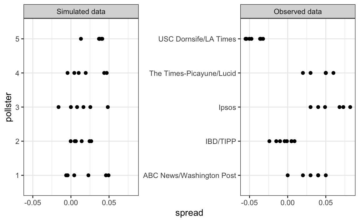
The model above does not account for pollster-to-pollster variability. To fix this, we add a new term for the pollster effect. We will use $h_i$ to represent the house effect of the $i$-th pollster. The model is now augmented to: 

$$
X_{i,j} = d + h_i + \varepsilon_{i,j}
$$

To simulate data from a specific pollster, we now need to draw an $h_i$ and then add the $\varepsilon$s. Here is how we would do it for one specific pollster. We assume $\sigma_h$ is 0.025:

```{r}
I <- 5
J <- 6
N <- 2000
d <- .021
p <- (d + 1) / 2
h <- rnorm(I, 0, 0.025)
X <- sapply(1:I, function(i){
  d + h[i] + rnorm(J, 0, 2 * sqrt(p * (1 - p) / N))
})
```

The simulated data now looks more like the actual data:
![plot2](https://rafalab.github.io/dsbook/book_files/figure-html/simulated-pollster-data-1.png)

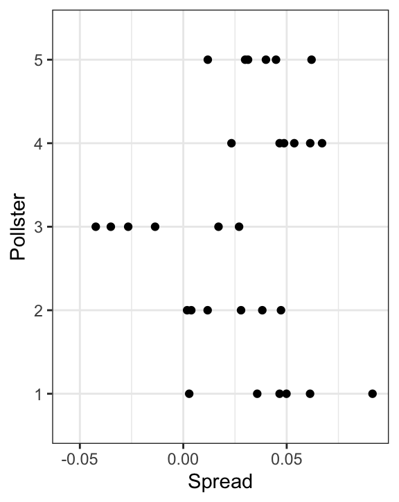
Note that $h_i$ is common to all the observed spreads from a specific pollster. Different pollsters have a different $h_i$, which explains why we can see the groups of points shift up and down from pollster to pollster.

Now, in the model above, we assume the average house effect is 0. We think that for every pollster biased in favor of our party, there is another one in favor of the other and assume the standard deviation is $\sigma_h$. But historically we see that every election has a general bias affecting all polls. 
We can observe this with the 2016 data, but if we collect historical data, we see that the average of polls misses by more than models like the one above predict. To see this, we would take the average of polls for each election year and compare it to the actual value. If we did this, we would see a difference with a standard deviation of between 2-3%. To incorporate this into the model, we can add another term to account for this variability:
$$
X_{i,j} = d + b + h_i + \varepsilon_{i,j}.
$$

Here $b$ is a random variable that accounts for the election-to-election variability. This random variable changes from election to election, but for any given election, it is the same for all pollsters and polls within on election. This is why it does not have indexes. This implies that all the random variables $X_{i,j}$ for an election year are correlated since they all have $b$ in common.

One way to interpret $b$ is as the difference between the average of all polls from all pollsters and the actual result of the election. Because we don't know the actual result until after the election, we can't estimate $b$ until after the election. However, we can estimate $b$ from previous elections and study the distribution of these values. Based on this approach we assume that, across election years, $b$ has expected value 0 and the standard error is about $\sigma_b = 0.025$. 

An implication of adding this term to the model is that the standard deviation for $X_{i,j}$ is actually higher than what we earlier called $\sigma$, which combines the pollster variability and the sample in variability, and was estimated with:

```{r}
sd(one_poll_per_pollster$spread)
```

This estimate does not include the variability introduced by $b$. Note that because

$$
\bar{X} = d + b + \frac{1}{N}\sum_{i=1}^N X_i,
$$

the standard deviation of $\bar{X}$ is:

$$
\sqrt{\sigma^2/N + \sigma_b^2}.
$$
Since the same $b$ is in every measurement, the average does not reduce the variability introduced by the $b$ term. This is an important point: it does not matter how many polls you take, this bias does not get reduced.

If we redo the Bayesian calculation taking this variability into account, we get a result much closer to FiveThirtyEight's:

```{r}
mu <- 0
tau <- 0.035
sigma <- sqrt(results$se^2 + .025^2)
Y <- results$avg
B <- sigma^2 / (sigma^2 + tau^2)
posterior_mean <- B*mu + (1-B)*Y
posterior_se <- sqrt( 1/ (1/sigma^2 + 1/tau^2))
1 - pnorm(0, posterior_mean, posterior_se)
```


### 16.8.4 Predicting the electoral college 

Up to now we have focused on the popular vote. But in the United States, elections are not decided by the popular vote but rather by what is known as the electoral college. Each state gets a number of electoral votes that depends, in a somewhat complex way, on the population size of the state. Here are the top 5 states ranked by electoral votes in 2016.

```{r}
results_us_election_2016 %>% top_n(5, electoral_votes)
```

With some minor exceptions we don't discuss, the electoral votes are won all or nothing. For example, if you win California by just 1 vote, you still get all 55 of its electoral votes. This means that by winning a few big states by a large margin, but losing many small states by small margins, you can win the popular vote and yet lose the electoral college. This happened in 1876, 1888, 2000, and 2016. The idea behind this is to avoid a few large states having the power to dominate the presidential election. Nonetheless, many people in the US consider the electoral college unfair and would like to see it abolished. 

We are now ready to predict the electoral college result for 2016. We start by aggregating results from a poll taken during the last week before the election. We use the `str_detect`, a function we introduce later in Section \@ref(stringr), to remove polls that are not for entire states. 

```{r}
results <- polls_us_election_2016 %>%
  filter(state!="U.S." & 
           !str_detect(state, "CD") & 
           enddate >="2016-10-31" & 
           (grade %in% c("A+","A","A-","B+") | is.na(grade))) %>%
  mutate(spread = rawpoll_clinton/100 - rawpoll_trump/100) %>%
  group_by(state) %>%
  summarize(avg = mean(spread), sd = sd(spread), n = n()) %>%
  mutate(state = as.character(state))
```

Here are the five closest races according to the polls:

```{r}
results %>% arrange(abs(avg))
```

We now introduce the command `left_join` that will let us easily add the number of electoral votes for each state from the dataset `us_electoral_votes_2016`. We will describe this function in detail in the Wrangling chapter. Here, we simply say that the function combines the two datasets so that the information from the second argument is added to the information in the first:

```{r}
results <- left_join(results, results_us_election_2016, by = "state")
```

Notice that some states have no polls because the winner is pretty much known:

```{r}
results_us_election_2016 %>% filter(!state %in% results$state) %>% 
  pull(state)
```

No polls were conducted in DC, Rhode Island, Alaska, and Wyoming because Democrats are  sure to win in the first two and Republicans in the last two.

Because we can't estimate the standard deviation for states with just one poll, we will estimate it as the median of the standard deviations estimated for states with more than one poll:

```{r}
results <- results %>%
  mutate(sd = ifelse(is.na(sd), median(results$sd, na.rm = TRUE), sd))
```

To make probabilistic arguments, we will use a Monte Carlo simulation. For each state, we apply the Bayesian approach to generate an election day $d$. We could construct the priors for each state based on recent history. However, to keep it simple, we assign a prior to each state that assumes we know nothing about what will happen. Since from election year to election year the results from a specific state don't change that much, we will assign a standard deviation of 2% or $\tau=0.02$. For now, we will assume, incorrectly, that the poll results from each state are independent. The code for the Bayesian calculation under these assumptions looks like this:

```{r}
mu <- 0
tau <- 0.02
results %>% mutate(sigma = sd/sqrt(n), 
                   B = sigma^2 / (sigma^2 + tau^2),
                   posterior_mean = B * mu + (1 - B) * avg,
                   posterior_se = sqrt(1/ (1/sigma^2 + 1/tau^2)))
```

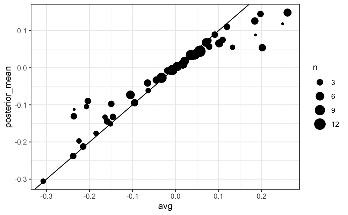
The estimates based on posterior do move the estimates towards 0, although the states with many polls are influenced less. This is expected as the more poll data we collect, the more we trust those results:
![geomabline](https://rafalab.github.io/dsbook/book_files/figure-html/posterior-versus-original-estimates-1.png)

Now we repeat this 10,000 times and generate an outcome from the posterior. In each iteration, we keep track of the total number of electoral votes for Clinton. Remember that Trump gets 270 minus the votes for Clinton. Also note that the reason we add 7 in the code is to account for Rhode Island and D.C.:

```{r}
B <- 10000
mu <- 0
tau <- 0.02
clinton_EV <- replicate(B, {
  results %>% mutate(sigma = sd/sqrt(n), 
                   B = sigma^2 / (sigma^2 + tau^2),
                   posterior_mean = B * mu + (1 - B) * avg,
                   posterior_se = sqrt(1 / (1/sigma^2 + 1/tau^2)),
                   result = rnorm(length(posterior_mean), 
                                  posterior_mean, posterior_se),
                   clinton = ifelse(result > 0, electoral_votes, 0)) %>% 
    summarize(clinton = sum(clinton)) %>% 
    pull(clinton) + 7
})
mean(clinton_EV > 269)
```

This model gives Clinton over 99% chance of winning. A similar prediction was made by the Princeton Election Consortium. We now know it was quite off. What happened?

The model above ignores the general bias and assumes the results from different states are independent. After the election, we realized that the general bias in 2016 was not that big: it was between 1 and 2%. But because the election was close in several big states and these states had a large number of polls, pollsters that ignored the general bias greatly underestimated the standard error. Using the notation we introduce, they assumed the standard error was $\sqrt{\sigma^2/N}$ which with large N is quite smaller than the more accurate estimate 
$\sqrt{\sigma^2/N + \sigma_b^2}$. FiveThirtyEight, which models the general bias in a rather sophisticated way, reported a closer result. We can simulate the results now with a bias term. For the state level, the general bias can be larger so we set it at $\sigma_b = 0.03$:


```{r}
tau <- 0.02
bias_sd <- 0.03
clinton_EV_2 <- replicate(1000, {
  results %>% mutate(sigma = sqrt(sd^2/n  + bias_sd^2),  
                   B = sigma^2 / (sigma^2 + tau^2),
                   posterior_mean = B*mu + (1-B)*avg,
                   posterior_se = sqrt( 1/ (1/sigma^2 + 1/tau^2)),
                   result = rnorm(length(posterior_mean), 
                                  posterior_mean, posterior_se),
                   clinton = ifelse(result>0, electoral_votes, 0)) %>% 
    summarize(clinton = sum(clinton) + 7) %>% 
    pull(clinton)
})
mean(clinton_EV_2 > 269)
```

This gives us a much more sensible estimate. Looking at the outcomes of the simulation, we see how the bias term adds variability to the final results.
![plot3](https://rafalab.github.io/dsbook/book_files/figure-html/comparison-forecast-with-and-without-bias-1.png)

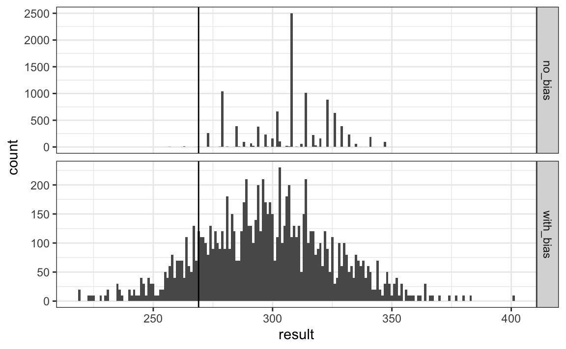
FiveThirtyEight includes many other features we do not include here.  One is that they model variability with distributions that have high probabilities for extreme events compared to the normal. One way we could do this is by changing the distribution used in the simulation from a normal distribution to a t-distribution. FiveThirtyEight predicted a probability of 71%.

### 16.8.5 Forecasting

Forecasters like to make predictions well before the election. The predictions are adapted as new polls come out. However, an important question forecasters must ask is: how informative are polls taken several weeks before the election about the actual election? Here we study the variability of poll results across time.


To make sure the variability we observe is not due to pollster effects, let's study data from one pollster:

```{r}
one_pollster <- polls_us_election_2016 %>% 
  filter(pollster == "Ipsos" & state == "U.S.") %>% 
  mutate(spread = rawpoll_clinton/100 - rawpoll_trump/100)
```

Since there is no pollster effect, then perhaps the theoretical standard error matches the data-derived standard deviation. We compute both here:

```{r}
se <- one_pollster %>% 
  summarize(empirical = sd(spread), 
            theoretical = 2 * sqrt(mean(spread) * (1 - mean(spread)) /
                                     min(samplesize)))
se
```

But the empirical standard deviation is higher than the highest possible theoretical estimate. Furthermore, the spread data does not look normal as the theory would predict:
![hist](https://rafalab.github.io/dsbook/book_files/figure-html/time-trend-variability-1.png)

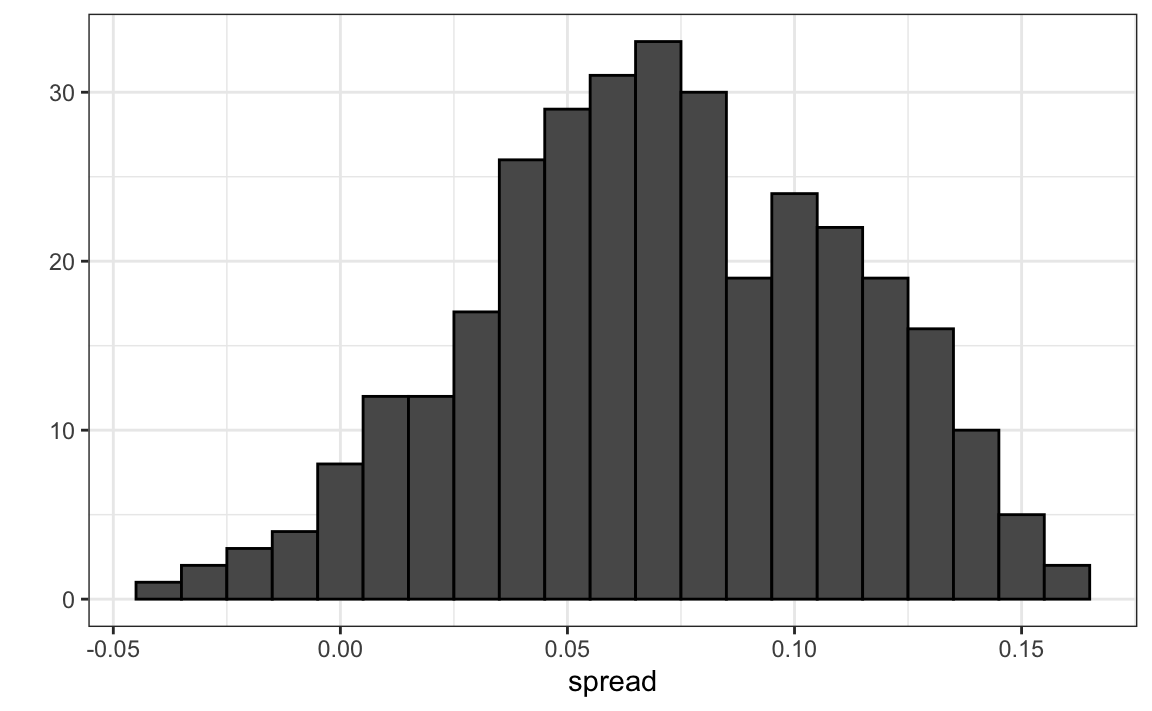
The models we have described include pollster-to-pollster variability and sampling error. But this plot is for one pollster and the variability we see is certainly not explained by sampling error. Where is the extra variability coming from? The following plots make a strong case that it comes from time fluctuations not accounted for by the theory that assumes $p$ is fixed:
![koool](https://rafalab.github.io/dsbook/book_files/figure-html/time-trend-estimate-1.png)

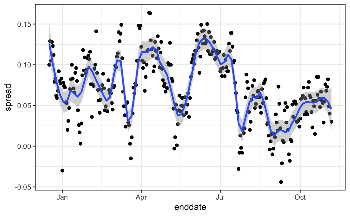
Some of the peaks and valleys we see coincide with events such as the party conventions, which tend to give the candidate a boost. We can see the peaks and valleys are consistent across several pollsters:
![doooope](https://rafalab.github.io/dsbook/book_files/figure-html/time-trend-estimate-several-pollsters-1.png)

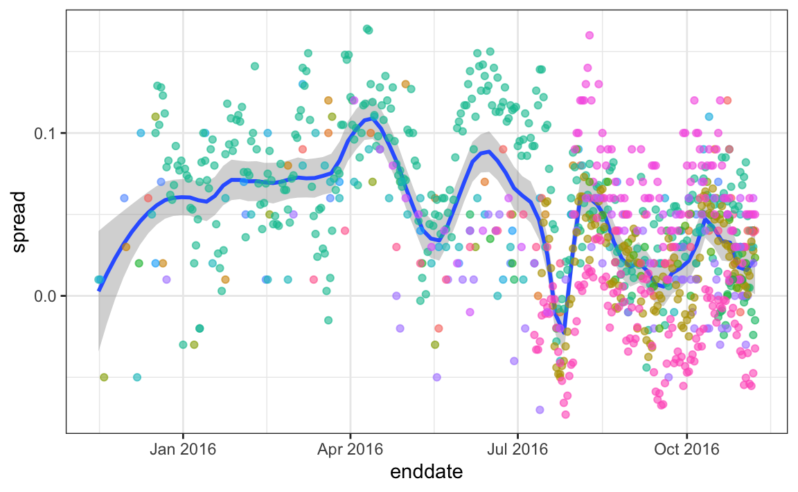
This implies that, if we are going to forecast, our model must include a term to accounts for the time effect. We need to write a model including a bias term for time:

$$
Y_{i,j,t} = d + b + h_j + b_t + \varepsilon_{i,j,t}
$$

The standard deviation of $b_t$ would depend on $t$ since the closer we get to election day, the closer to 0 this bias term should be. 

Pollsters also try to estimate trends from these data and incorporate these into their predictions. We can model the time trend with a function $f(t)$ and rewrite the model like this:
The blue lines in the plots above: 


$$
Y_{i,j,t} = d + b + h_j + b_t + f(t) + \varepsilon_{i,jt,}
$$

We usually see the estimated $f(t)$ not for the difference, but for the actual percentages for each candidate like this:
![daaaaaang](https://rafalab.github.io/dsbook/book_files/figure-html/trend-estimate-for-all-pollsters-1.png)

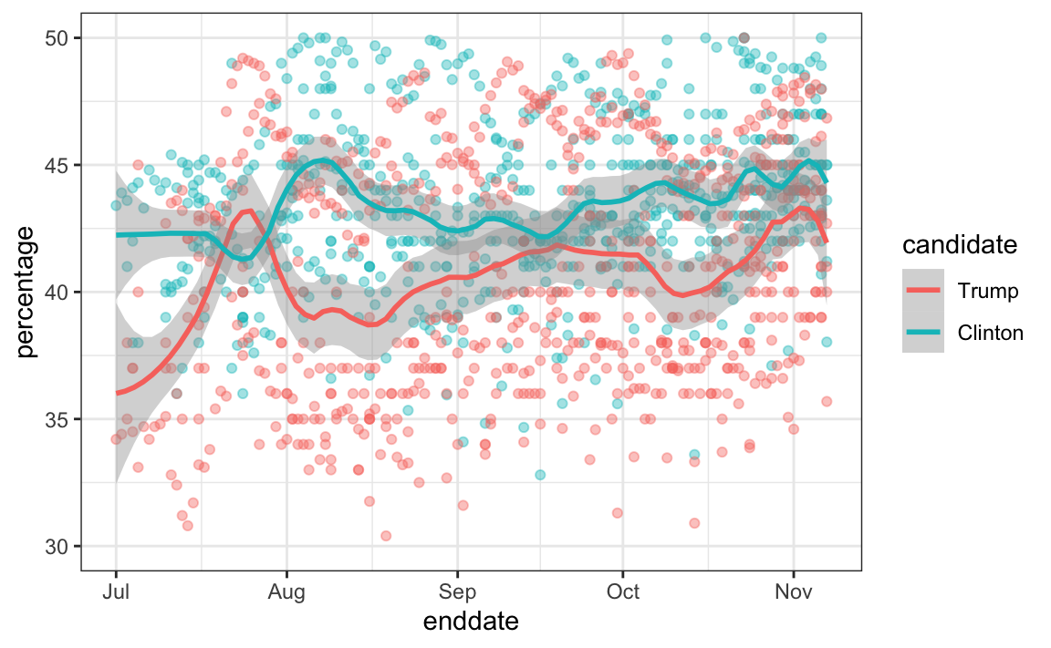
Once a model like the one above is selected, we can use historical and present data to estimate all the necessary parameters to make predictions. There is a variety of methods for estimating trends $f(t)$ which we discuss in the Machine Learning part.

# 16.9 Exercises

1\. Create this table:

```{r}
library(tidyverse)
library(dslabs)
data("polls_us_election_2016")
polls <- polls_us_election_2016 %>% 
  filter(state != "U.S." & enddate >= "2016-10-31") %>% 
  mutate(spread = rawpoll_clinton/100 - rawpoll_trump/100)
```

Now for each poll use the CLT to create a 95% confidence interval for the spread reported by each poll. Call the resulting object cis with columns lower and upper for the limits of the confidence intervals. Use the `select` function to keep the columns `state, startdate, end date, pollster, grade, spread, lower, upper`.
```{r}
cis <- polls %>% mutate(X_hat = (spread+1)/2, se = 2*sqrt(X_hat*(1-X_hat)/samplesize), 
                 lower = spread - qnorm(0.975)*se, upper = spread + qnorm(0.975)*se) %>%
  select(state, startdate, enddate, pollster, grade, spread, lower, upper)
```

2\. You can add the final result to the `cis` table you just created using the `right_join` function like this:

```{r}
add <- results_us_election_2016 %>% 
  mutate(actual_spread = clinton/100 - trump/100) %>% 
  select(state, actual_spread)
cis <- cis %>% 
  mutate(state = as.character(state)) %>% 
  left_join(add, by = "state")
```

Now determine how often the 95% confidence interval includes the actual result.
```{r}
p_hits <- cis %>% mutate(hit = lower <= actual_spread & upper >= actual_spread) %>% summarize(proportion_hits = mean(hit))
p_hits
```


3\. Repeat this, but show the proportion of hits for each pollster. Show only pollsters with more than 5 polls and order them from best to worst. Show the number of polls conducted by each pollster and the FiveThirtyEight grade of each pollster. Hint: use `n=n(), grade = grade[1]` in the call to summarize.
```{r}
p_hits <- cis %>% mutate(hit = lower <= actual_spread & upper >= actual_spread) %>% 
  group_by(pollster) %>%
  filter(n() >=  5) %>%
  summarize(proportion_hits = mean(hit), n = n(), grade = grade[1]) %>%
  arrange(desc(proportion_hits))
p_hits
```


4\. Repeat exercise 3, but instead of pollster, stratify by state. Note that here we can't show grades. 
```{r}
p_hits <- cis %>% mutate(hit = lower <= actual_spread & upper >= actual_spread) %>% 
  group_by(state) %>%
  filter(n() >=  5) %>%
  summarize(proportion_hits = mean(hit), n = n()) %>%
  arrange(desc(proportion_hits)) 
p_hits
```


5\. Make a barplot based on the result of exercise 4. Use `coord_flip`.
```{r fig.height=9, fig.width=16}
p_hits %>% mutate(state = reorder(state, proportion_hits)) %>%
  ggplot(aes(state, proportion_hits)) + 
  geom_bar(stat = "identity") +
  coord_flip()
```



6\. Add two columns to the `cis` table by computing, for each poll, the difference between the predicted spread and the actual spread, and define a column `hit` that is true if the signs are the same. Hint: use the function `sign`. Call the object `resids`.
```{r}
resids <- cis %>% mutate(error = spread - actual_spread, hit = sign(spread) == sign(actual_spread))
resids
```


7\. Create a plot like in exercise 5, but for the proportion of times the sign of the spread agreed.
```{r fig.height=9, fig.width=16}
p_hits <- resids %>%  group_by(state) %>%
  filter(n() >=  5) %>%
  summarize(proportion_hits = mean(hit), n = n())

p_hits %>% mutate(state = reorder(state, proportion_hits)) %>%
  ggplot(aes(state, proportion_hits)) + 
  geom_bar(stat = "identity") +
 coord_flip()
```


8\. In exercise 7, we see that for most states the polls had it right 100% of the time. For only 9 states did the polls miss more than 25% of the time. In particular, notice that in Wisconsin every single poll got it wrong. In Pennsylvania and Michigan more than 90% of the polls had the signs wrong. Make a histogram of the errors. What is the median of these errors?
```{r}
hist(resids$error)
median(resids$error)
```


9\. We see that at the state level, the median error was 3% in favor of Clinton. The distribution is not centered at 0, but at 0.03. This is the general bias we described in the section above. Create a boxplot to see if the bias was general to all states or it affected some states differently. Use `filter(grade %in% c("A+","A","A-","B+") | is.na(grade))) ` to only include pollsters with high grades.
```{r fig.height=9, fig.width=16}
resids %>% filter(grade %in% c("A+","A","A-","B+") | is.na(grade)) %>%
  mutate(state = reorder(state, error)) %>%
  ggplot(aes(state, error)) + 
  theme(axis.text.x = element_text(angle = 90, hjust = 1)) +
  geom_boxplot() + 
  geom_point()
```


10\. Some of these states only have a few polls. Repeat exercise 9, but only include states with 5 good polls or more. Hint: use `group_by`, `filter` then `ungroup`. You will see that the West (Washington, New Mexico, California) underestimated Hillary's performance, while the Midwest (Michigan, Pennsylvania, Wisconsin, Ohio, Missouri) overestimated it. In our simulation, we did not model this behavior since we added general bias, rather than a regional bias. Note that some pollsters may now be modeling correlation between similar states and estimating this correlation from historical data. To learn more about this, you can learn about random effects and mixed models.
```{r}
resids %>% filter(grade %in% c("A+","A","A-","B+") | is.na(grade)) %>%
  group_by(state) %>%
  filter(n() >= 5) %>%
  ungroup() %>%
  mutate(state = reorder(state, error)) %>%
  ggplot(aes(state, error)) + 
  theme(axis.text.x = element_text(angle = 90, hjust = 1)) +
  geom_boxplot() + 
  geom_point()
```

# 16.10 The t-distribution

Above we made use of the CLT with a sample size of 15. Because we are estimating a second parameters $\sigma$, further variability is introduced into our confidence interval which results in intervals that are too small. For very large sample sizes this extra variability is negligible, but, in general, for values smaller than 30 we need to be cautious about using the CLT. 

However, if the data in the urn is known to follow a normal distribution, then we actually have mathematical theory that tells us how much bigger we need to make the intervals to account for the estimation of $\sigma$. Using this theory, we can construct confidence intervals for any $N$. But again, this works only if **the data in the urn is known to follow a normal distribution**. So for the 0, 1 data of our previous urn model, this theory definitely does not apply.

The statistic on which confidence intervals for $d$ are based is

$$
Z = \frac{\bar{X} - d}{\sigma/\sqrt{N}}
$$

CLT tells us that Z is approximately normally distributed with expected value 0 and standard error 1. But in practice we don't know $\sigma$ so we use:

$$
Z = \frac{\bar{X} - d}{s/\sqrt{N}}
$$


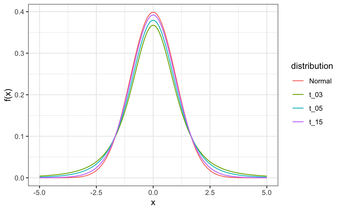
By substituting $\sigma$ with $s$ we introduce some variability. The theory tells us that $Z$ follows a t-distribution with $N-1$ _degrees of freedom_. The degrees of freedom is a parameter that controls the variability via fatter tails:
![colors](https://rafalab.github.io/dsbook/book_files/figure-html/t-distribution-examples-1.png)

If we are willing to assume the pollster effect data is normally distributed, based on the sample data $X_1, \dots, X_N$,  
```{r}
one_poll_per_pollster %>%
  ggplot(aes(sample=spread)) + stat_qq()
```
then $Z$ follows a t-distribution with $N-1$ degrees of freedom. So perhaps a better confidence interval for $d$ is:


```{r}
z <- qt(0.975,  nrow(one_poll_per_pollster)-1)
one_poll_per_pollster %>% 
  summarize(avg = mean(spread), moe = z*sd(spread)/sqrt(length(spread))) %>% 
  mutate(start = avg - moe, end = avg + moe) 
```

A bit larger than the one using normal is 

```{r}
qt(0.975, 14)
```

is bigger than

```{r}
qnorm(0.975)
```

The t-distribution can also be used to model errors in bigger deviations that are more likely than with the normal distribution, as seen in the densities we previously saw. Fivethirtyeight uses the t-distribution to generate errors that better model the deviations we see in election data. For example, in Wisconsin the average of six polls was 7% in favor of Clinton with a standard deviation of 1%, but Trump won by 0.7%. Even after taking into account the overall bias, this 7.7% residual is more in line with t-distributed data than the normal distribution.

```{r}
data("polls_us_election_2016")
polls_us_election_2016 %>%
  filter(state =="Wisconsin" &
           enddate >="2016-10-31" & 
           (grade %in% c("A+","A","A-","B+") | is.na(grade))) %>%
  mutate(spread = rawpoll_clinton/100 - rawpoll_trump/100) %>%
  mutate(state = as.character(state)) %>%
  left_join(results_us_election_2016, by = "state") %>%
  mutate(actual = clinton/100 - trump/100) %>%
  summarize(actual = first(actual), avg = mean(spread), 
            sd = sd(spread), n = n()) %>%
  select(actual, avg, sd, n)
```