-
Notifications
You must be signed in to change notification settings - Fork 0
/
Copy pathvignette_SimpleFlow.Rmd
368 lines (299 loc) · 15.2 KB
/
vignette_SimpleFlow.Rmd
1
2
3
4
5
6
7
8
9
10
11
12
13
14
15
16
17
18
19
20
21
22
23
24
25
26
27
28
29
30
31
32
33
34
35
36
37
38
39
40
41
42
43
44
45
46
47
48
49
50
51
52
53
54
55
56
57
58
59
60
61
62
63
64
65
66
67
68
69
70
71
72
73
74
75
76
77
78
79
80
81
82
83
84
85
86
87
88
89
90
91
92
93
94
95
96
97
98
99
100
101
102
103
104
105
106
107
108
109
110
111
112
113
114
115
116
117
118
119
120
121
122
123
124
125
126
127
128
129
130
131
132
133
134
135
136
137
138
139
140
141
142
143
144
145
146
147
148
149
150
151
152
153
154
155
156
157
158
159
160
161
162
163
164
165
166
167
168
169
170
171
172
173
174
175
176
177
178
179
180
181
182
183
184
185
186
187
188
189
190
191
192
193
194
195
196
197
198
199
200
201
202
203
204
205
206
207
208
209
210
211
212
213
214
215
216
217
218
219
220
221
222
223
224
225
226
227
228
229
230
231
232
233
234
235
236
237
238
239
240
241
242
243
244
245
246
247
248
249
250
251
252
253
254
255
256
257
258
259
260
261
262
263
264
265
266
267
268
269
270
271
272
273
274
275
276
277
278
279
280
281
282
283
284
285
286
287
288
289
290
291
292
293
294
295
296
297
298
299
300
301
302
303
304
305
306
307
308
309
310
311
312
313
314
315
316
317
318
319
320
321
322
323
324
325
326
327
328
329
330
331
332
333
334
335
336
337
338
339
340
341
342
343
344
345
346
347
348
349
350
351
352
353
354
355
356
357
358
359
360
361
362
363
364
365
366
367
---
title: "Vignette - Simple Flow"
author: "Julie Chuong"
date: "4/3/2022"
output:
html_notebook: default
pdf_document: default
html_document: default
---
This notebook is to show you how to use the package CytoexploreR to analyze flow cytometry data from the Cytek Aurora.
This vignette is worthwhile if you have only one or two flow datasets, like checking samples of GFP-tagged strains for GFP, viability stains of cells, etc.
We do not recommend this vignette for timecourse data, ie. multiple subdirectories of flow data, wherein there is one subdirectory for each sampling day.
For a vignette that analyzes timecourse flow data, see the our Vignette - Timecourse Flow.
### Install CytoExplorer package and requirements. Skip if already installed.
```{r include = FALSE}
require("knitr")
knitr::opts_chunk$set(eval = FALSE, echo = TRUE, message = FALSE, warning = FALSE)
```
```{r}
library(BiocManager)
install.packages("cytolib", "flowCore", "flowWorkspace", "openCyto")
```
Install CytoExploreR from GitHub. Skip is already installed.
```{r}
library(devtools)
devtools::install_github("DillonHammill/CytoExploreR")
```
Load required packages
```{r}
library(CytoExploreR)
library(tidyverse)
library(ggridges)
```
## Vignette Dataset
There were four samples that were analyzed on the Cytek Aurora.
One was *GAP1* CNV reporter strain (DGY1657), in which a mCitrine gene was inserted upstream of the *GAP1* promoter
and coding sequence. Additionally, there was one sample each of 3 control strains: zero copy 'unstained' control
(DGY1) that has no mCitrine, one copy control (DGY500) in which the mCitrine gene was inserted in neutral locus, HO,
that doesn't undergo copy number variation under glutamine-limited growth, and two copy control (DGY1315) containing
two inserted copies of mCitrine in neutral loci. Each sample was cultured from a single colony overnight in
glutamine-limited media at 30C.
In each sample, 100,000 events were measured on the Cytek Aurora Flow Cytometer for mCitrine fluorescence
(excitation wavelength = 516, emission wavelength = 529 ) via the B2-A channel, forward scatter (FSC), and
side scatter (SSC).
Note that you may have used a different channel depending on your cell stain.
## Set working directory
Place your FCS files in a directory. Multiple subdirectories containing FCS files are OK.
**Note 1**: You can only load in one folder's worth of FCS files at a time. In this vignette,
we put all of our FCS data files in one subdirectory named FCS_files. There is one FSC file per sample.
In total, there are 4 FSC files.
**Note 2**: You should **NOT** manually rename your FCS files after exporting it from the Cytek.
In other words, files should have their original names from the machine.
"Renaming the files manually is not recommended as it does not update the associated keywords contained in the FCS files"
(Source: https://github.com/DillonHammill/CytoExploreR/issues/85). If files need to renamed, do so on on the Cytek
software and re-export the FCS files.
```{r setup, results='asis'}
require("knitr")
knitr::opts_knit$set(root.dir = "~/Documents/vignette_simple_data_workingcopy")
```
```{r include = TRUE}
getwd()
```
## Version name
Choose a name to be used for all output files including the gatingTemplate.csv and associated flow data and graphs.
In this vignette, we will set it to my initials, date, and version 1.
```{r}
version_name = "my_initials_date_v1"
```
## STEP 1: Load in FCS data as a gating set
**INSTRUCTIONS**:
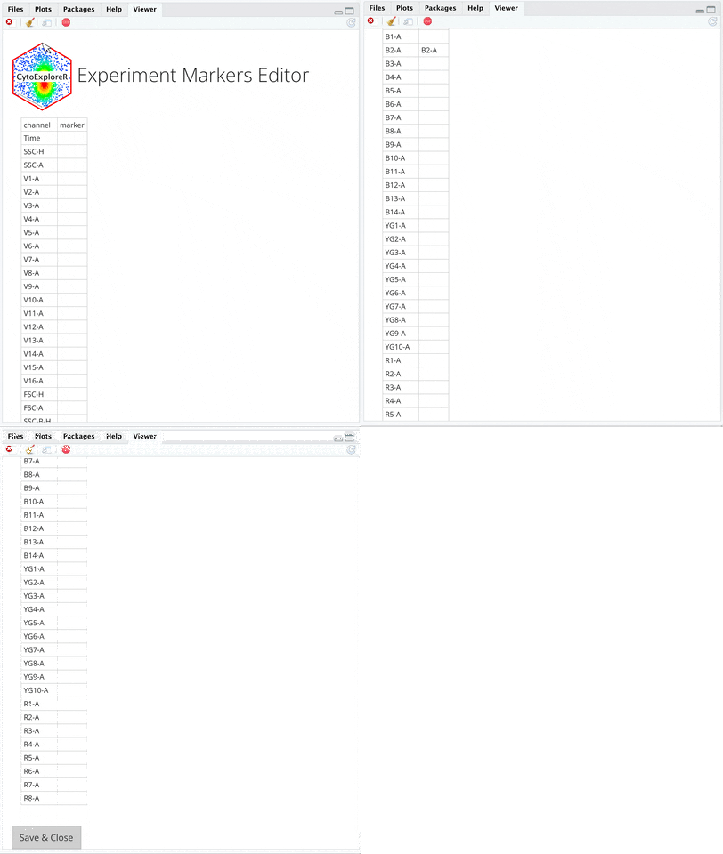
+ An editable markers sheet will show up on `Viewer` Pane.
+ Edit Markers on Viewer pane by typing in "B2-A" in the `marker` column of the B2-A channel. FSC and SSC are included markers by default so you do not need to edit them.
+ Scroll to the bottom of the Viewer pane.
+ Click `Save & Close` button at the bottom of the `Viewer` pane.

```{r}
my_gating_set <- cyto_setup(path = "./FCS_files", restrict=TRUE, select="fcs")
```
## STEP 2: Edit the experimental details to include metadata from the sample sheet
Merge samplesheet with autogenerated experiment details file generated from `cyto_setup()`.
**ONLY NEED TO DO ONCE** to generate `Vignette-Experiment-Details.csv` file. Once you have the file, it will automatically be used the next time you load in FCS data as a gating set (STEP 1).
Here we assume the samplesheet metadata file is already in the working directory.
Provide the file path to the sample sheet (metadata).
```{r}
file.rename(dir(pattern = "Experiment-Details.csv"),"Vignette-Experiment-Details.csv")
exp_details = read_csv(file = paste0(list.files(pattern = "Experiment-Details.csv")))
sample_sheet = read_csv(file = paste0(list.files(pattern = "sample_sheet_vignette_simple.csv")))
experiment_details = left_join(exp_details, sample_sheet) %>%
write_csv("Vignette-Experiment-Details.csv")
```
Add the experiment details metadata to the gating set.
**ONLY NEED TO ONCE**
```{r}
for(i in 1:length(names(experiment_details))){
flowWorkspace::pData(my_gating_set)[names(experiment_details[i])]<-experiment_details[i]
}
```
Check that the experiment details metadata were successfully attached to the gating set.
```{r}
cyto_details(my_gating_set)
```
By default the Experiment-Markers.csv file is named with the date created.
Rename the autogenerated experiment-markers.csv file.
**ONLY NEED TO DO ONCE**
```{r}
file.rename(dir(pattern = "Experiment-Markers.csv"),"Vignette-Experiment-Markers.csv")
```
## STEP 3: Perform gating on gating set
Gate for 1) Cells, 2) Singlets, 3) CNVS
Results in a gating file and gated data.
**Transform the data**
Transforming the data makes it easier to interpret visually and well as to draw gates.
For this vignette's data, when the transformed data are plotted, the zero copy strains take up most of the coordinate plane and the one copy and two copy distributions are very close together. The fluorescence profiles/distributions of the one copy and two copy controls overlap some. They are not mutually exclusive which is a limitation to note.
This is a useful article if you I want think about to choosing different transformations:
https://dillonhammill.github.io/CytoExploreR/articles/CytoExploreR-Transformations.html
In our case, it was necessary to use a logicle transformation for the `B2-A` values and then
a log transformation for the other values. I could not use `logicle transformation` nor could I use the `log transformation` for all values.
**IMPORTANT**: If you get an error message*, run the in the Console, not inside the R notebook. Make sure you reset your working directory in the Console.
*Error in plot.new() : QuartzBitmap_Output - unable to open file
```{r}
GFP_trans <- cyto_transformer_logicle(my_gating_set,
channels = c("B2-A"),
widthBasis = -10
)#returns it as a list
FSC_SSC_trans <- cyto_transformer_log(my_gating_set,
channels = c("FSC-A", "FSC-H", "SSC-A", "SSC-H")
) #log transform the forward and side scatter
combined_trans <- cyto_transformer_combine(GFP_trans,FSC_SSC_trans) #combine both transformations
transformed_gating_set <- cyto_transform(my_gating_set,
trans = combined_trans) #applies the the transformation and returns it as a gatingSet
```
Check the transformed data by plotting
```{r}
cyto_plot_explore(transformed_gating_set, #plots all FCS files
channels_x = "FSC-A",
channels_y = "B2-A",
axes_limits = "data")
```
Subset rows to plot as desired, using the row assignment in `cyto_details()`
```{r}
cyto_details(transformed_gating_set)
cyto_plot_explore(transformed_gating_set[c(2,3)], #here we specify to plot rows 2 and 3
channels_x = "FSC-A",
channels_y = "B2-A",
axes_limits = "data")
```
### Draw Gates using Control Strains as a Guide
**Note**: if you already have a gating template and don't need to draw gates, skip the `cyto_gate_draw()` steps.
Instead, use `cyto_gatingTemplate_apply()` to apply a `gatingTemplate.csv` to your gating set.
```{r}
cyto_gatingTemplate_apply(transformed_gating_set, gatingTemplate=paste0( "cytek_gating_",version_name,".csv"))
```
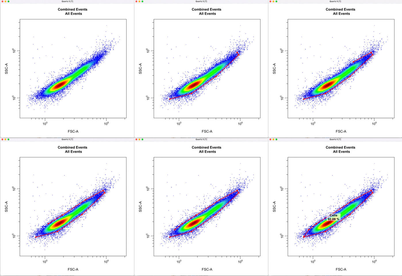
##### To Draw Gates
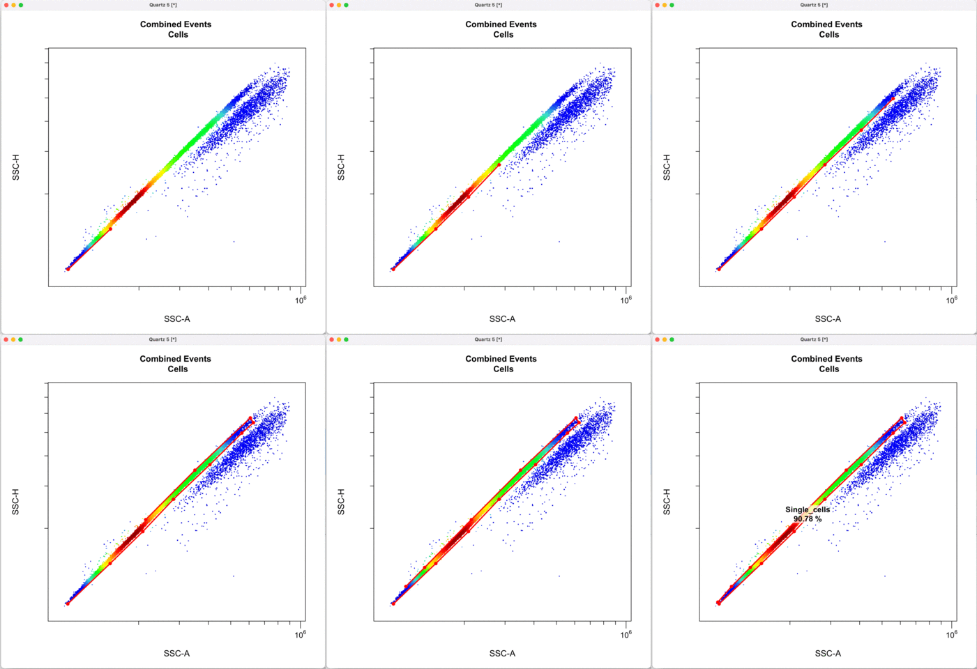
**INSTRUCTIONS**
* A new window will pop out.
* Draw the desired gate.
* Press `esc` on keyboard when finished drawing to save the gate.
* Gating coordinates will be placed in a gatingTemplate.csv file which can be applied (without drawing again) in future code runs.
First we gate for the cells, filtering out cell debris, bacteria, etc.
```{r}
cyto_gate_draw(transformed_gating_set,
parent = "root",
alias = "Cells",
channels = c("FSC-A","SSC-A"),
axes_limits = "data",
gatingTemplate = paste0("cytek_gating_",version_name,".csv")
)
```

Then we define the singlets based on side-scatter area and height.
See other ways to discriminate doublets: https://expert.cheekyscientist.com/how-to-perform-doublet-discrimination-in-flow-cytometry/
```{r}
cyto_gate_draw(transformed_gating_set,
parent = "Cells",
alias = "Single_cells",
channels = c("SSC-A","SSC-H"),
axes_limits = "data",
gatingTemplate = paste0("cytek_gating_",version_name,".csv")
)
```

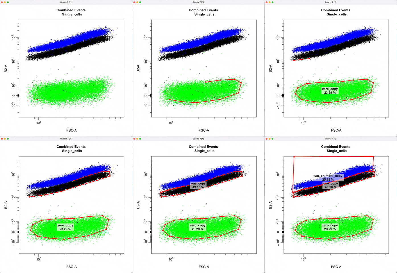
Gating for CNVs using the 0,1 and 2 copy controls:
In `cyto_extract()`, we can subset and extract the rows of interest. Here, we use `cyto_extract()` to
extract the 0, 1, and 2 copy control populations in order to overlay them on a plot when drawing gates.
The row assignment correspond to the experimental details associated with the gating set.
In `cyto_gate_draw()`, choose colors of the parent population and the overlay populations.
In `cyto_date_draw()`, the `alias` argument lets you choose gate names.
```{r}
cyto_details(transformed_gating_set) #View the rows and choose which to extract
```
```{r}
zero_ctrl <- cyto_extract(transformed_gating_set, "Single_cells")[c(1)] # row of 0 copy control data
one_ctrl <- cyto_extract(transformed_gating_set, "Single_cells")[c(2)] # row of 1 copy control data
two_ctrl <- cyto_extract(transformed_gating_set, "Single_cells")[c(4)] # row of 2 copy control data
cyto_gate_draw(transformed_gating_set,
point_col = c("gray", "green", "black", "blue"), #choose colors
parent = "Single_cells", #maps to first point color
overlay = c(zero_ctrl, one_ctrl, two_ctrl),#maps to remaining point colors
alias = c("zero_copy", "one_copy", "two_or_more_copy"), #Name the gate names here
channels = c("FSC-A","B2-A"),
axes_limits = "data",
gatingTemplate = paste0("cytek_gating_",version_name,".csv")
)
```

## STEP 4: Get statistics
Get cell counts in each gate
```{r}
counts = gs_pop_get_stats(transformed_gating_set, c("Single_cells", "zero_copy", "one_copy", "two_or_more_copy")) %>%
rename(Gate = pop, name = sample, Count = count) %>%
left_join(experiment_details) %>%
write_csv(paste0(version_name,"_counts.csv"))
#counts = read_csv(paste0(version_name,"_counts.csv"))
```
Get frequency of cells inside each gate
```{r}
freq = gs_pop_get_stats(transformed_gating_set, c("Single_cells","zero_copy", "one_copy", "two_or_more_copy"), type = "percent") %>%
rename(Gate = pop, name = sample, Frequency = percent) %>%
left_join(experiment_details) %>%
write_csv(paste0(version_name,"_freq.csv"))
#freq = read_csv(paste0(version_name,"_freq.csv"))
```
Check that there are at least 70,000 single cells per sample
```{r}
freq_and_counts =
counts %>% filter(Gate == "Single_cells") %>%
rename(Parent = Gate) %>%
left_join(freq) %>%
filter(!(Gate == "Single_cells")) %>%
mutate(Frequency = Frequency*100) %>%
relocate(2:3, .after = Gate)
```
```{r}
freq_and_counts %>%
distinct(Strain, Count)
```
Plot frequency of cells in gates per sample
```{r}
freq_bar = freq_and_counts %>%
mutate(Gate = fct_relevel(Gate, c("zero_copy", "one_copy", "two_or_more_copy")),
Strain=fct_relevel(Strain, c("DGY1","DGY500","DGY1657","DGY1315")),
Description=fct_relevel(Description, c("0 copy control", "1 copy control","CNV reporter strain","2 copy control"))
)%>%
filter(Count>70000) %>%
ggplot(aes(Description, Frequency, fill = Gate)) +
geom_bar(position="dodge", stat="identity") +
scale_fill_manual(values= c(RColorBrewer::brewer.pal(3, "Greens"))) +
ylab("% of cells in gate") +
theme_classic() +
theme(text = element_text(size=12))
freq_bar
```
Get raw transformed `B2-A` and `FSC` values for every cell
```{r}
timepoint_raw_list <- cyto_extract(transformed_gating_set, parent = "Single_cells", raw = TRUE, channels = c("FSC-A", "B2-A")) #raw flow data of each cell as a list of matrices
sc_distr = map_df(timepoint_raw_list, ~as.data.frame(.x), .id="name") %>% #convert to df, put list name in new column
left_join(experiment_details) %>% #join by name column to add metadata
mutate(B2A_FSC = `B2-A`/`FSC-A`) %>% #compute normalized fluorescence for every cell
write_csv(paste0(version_name,"_SingleCellDistributions.csv"))
sc_distr = read_csv(paste0(version_name,"_SingleCellDistributions.csv"))
```
## STEP 5: Make Plots
**Graph single cell fluorescence distributions (ridgeplots) for each sample**
```{r}
sc_distr = sc_distr %>%
mutate_if(is.character,as.factor) %>% #change all strings columns to factors
mutate(Strain=fct_relevel(Strain,c("DGY1","DGY500","DGY1657","DGY1315")),
`mCitrine copy number`=fct_relevel(`mCitrine copy number`, c("zero copy","one copy", "two copy" )),
Description=fct_relevel(Description, c("0 copy control", "1 copy control","CNV reporter strain","2 copy control"))
)
sc_distr %>%
ggplot(aes(B2A_FSC, Description, fill = `mCitrine copy number`)) +
geom_density_ridges(scale = 1) +
scale_y_discrete(expand = expansion(add = c(0.2, 1.0)))+
scale_fill_manual(values= c(RColorBrewer::brewer.pal(3, "Greens"))) +
scale_x_continuous("normalized fluorescence", limits=c(0, 3.0), breaks = c(0, 1, 2, 3), labels = c(0,1,2,3)) +
theme_classic() +
theme(
axis.text.x = element_text(family="Arial", size = 10, color = "black"), #edit x-tick labels
axis.text.y = element_text(family="Arial", size = 10, color = "black"),
strip.background = element_blank(), #remove box around facet title
strip.text = element_text(size=12)
)
```
**Graph boxplots of normalized fluorescence per sample**
```{r echo=TRUE}
ggplot(sc_distr, aes(Strain, B2A_FSC, fill = `mCitrine copy number`)) +
geom_boxplot() +
ylab("normalized fluorescence")+
scale_fill_manual(values= c(RColorBrewer::brewer.pal(3, "Greens"))) +
theme_classic() +
theme(
#legend.position = 'none', #remove the legend
axis.text.x = element_text(family="Arial", size = 10, color = "black"), #edit x-tick labels
axis.text.y = element_text(family="Arial", size = 10, color = "black"),
strip.background = element_blank(), #remove box around facet title
strip.text = element_text(size=12)
)
```